How elections are impacted by a 100 million year old coastline
How elections are impacted by a 100 million year old coastline
Earth Science and Geology impact American social and political life in unexpected ways
Hale County in west central Alabama and Bamberg County in southern South Carolina are 450 miles apart. Both counties have a population of 16,000 of which around 60% are African American. The median households and per capita incomes are well below their respective state’s median, in Hale nearly $10,000 less. Both were named after confederate officers–Stephen Fowler Hale and Francis Marion Bamberg. And although Hale’s county seat is the self-proclaimed Catfish Capitol, pulling catfish out of the Edisto River in Bamberg County is a favorite past time.
These two counties share another unique feature. Amidst a blanket of Republican red both Hale and Bamberg voted primarily Democratic in the 2000, 2004, and again in the 2008 presidential elections. Indeed, Hale and Bamberg belong to a belt of counties cutting through the deep south–Mississippi, Alabama, Georgia, South Carolina, and North Carolina–that have voted over 50% Democratic in recent presidential elections.
Why? A 100 million year old coastline.

During the Cretaceous, 139-65 million years ago, shallow seas covered much of the southern United States. These tropical waters were productive–giving rise to tiny marine plankton with carbonate skeletons which overtime accumulated into massive chalk formations. The chalk, both alkaline and porous, lead to fertile and well-drained soils in a band, mirroring that ancient coastline and stretching across the now much drier South. This arc of rich and dark soils in Alabama has long been known as the Black Belt.
But many, including Booker T. Washington, coopted the term to refer to the entire Southern band. Washington wrote in his 1901 autobiography, Up from Slavery, “The term was first used to designate a part of the country which was distinguished by the color of the soil. The part of the country possessing this thick, dark, and naturally rich soil…”

Over time this rich soil produced an amazingly productive agricultural region, especially for cotton. In 1859 alone a harvest of over 4,000 cotton bales was not uncommon within the belt. And yet, just tens of miles north or south this harvest was rare. Of course this level of cotton production required extensive labor.

As Washington notes further in his autobiography, “The part of the country possessing this thick, dark, and naturally rich soil was, of course, the part of the South where the slaves were most profitable, and consequently they were taken there in the largest numbers. Later and especially since the war, the term seems to be used wholly in a political sense—that is, to designate the counties where the black people outnumber the white.”

The legacy of ancient coastlines, chalk, soil, cotton, and slavery can still be seen today. African Americans make up over 50%, in some cases over 85%, of the population in Black Belt counties. As expected this has and continues to deeply influence the culture of the Black Belt. J. Sullivan Gibson writing in 1941 on the geology of the Black Belt noted, “The long-conceded regional identity of the Black Belts roots no more deeply its physical fundament of rolling prairie soil than in its cultural, social, and economic individuality.” And so this plays out in politics.

This Black Belt with its predominantly African American population consistently votes overwhelmingly for Democratic candidates in presidential elections. The pattern is especially pronounced on maps when a Republican candidate has secured the presidency as Bush did in 2000 and 2004. In Southern states where a Republican secures the nomination, almost the entirety of Black Belt counties still lean Democratic. This leads to a Blue Belt of Democratic counties across the South. Even when Clinton, a Democrat, overwhelmingly took most Southern states, the percentages of those voting Democrat was still highest in the Black Belt counties.

But the Black Belt has not always been visible on maps during elections. The Voting Rights Act, outlawing discriminatory voting practices, was passed in 1965. As result, a year earlier in the 1964 elections larger numbers of African Americans were excluded from the polls in Southern states. And, in turn, the blue band we see today was not visible.
Long heralded as the Black Belt for rich dark soils and later for the rich African American culture and population, it may equally be referred to as the Blue Belt to reflect both its oceanic geology and the political leanings that resulted from it.
About the author: Craig McClain is the Executive Director of the Lousiana University Marine Consortium. He has conducted deep-sea research for 20 years and published over 50 papers in the area. He has participated in and led dozens of oceanographic expeditions taken him to the Antarctic and the most remote regions of the Pacific and Atlantic.
Deep Sea News: How presidential elections are impacted by a 100 million year old coastline
– – – – – – – – – – – – – – –
Now we move to further data, from the original article, Geology and Election 2000: Overview, by Steven Dutch, Natural and Applied Sciences,University of Wisconsin – Green Bay
On the map of electoral returns for the presidential election of 2000 is a feature instantly recognizable to a geologist: in the otherwise pro-Bush South, an arcuate band of pro-Gore counties sweeps from eastern Mississippi, across Alabama and Georgia and into the Carolinas.

My geologist’s eye was immediately drawn to this arc because it coincides almost exactly with a series of rock units on the Geologic Map of the United States. Why would election returns follow rock outcrops?
In the map below, Cretaceous rock units (139-65 million years old) are shown in shades of green. Older rock units are in gray, younger ones in yellow. The complex NE-trending patterns in Alabama, Georgia and South Carolina are deformed rocks of the Appalachians. In NW Alabama, the older rocks are flat-lying layers of the continental interior.
Comparison with the geologic maps shows that the arc actually consists of three segments.
- In Mississippi and Alabama the pro-Gore band of counties corresponds very closely with the units labeled uK – upper Cretaceous. We might suspect that the most likely explanation for this part of the arc has to do with economic patterns dictated by the soils. Most of the electoral and demographic patterns associated with the band end abruptly in NE Mississippi.
- In Georgia, the Cretaceous outcrop band is very narrow. It is surprising how clear the pro-Gore band is in Georgia considering how narrow and discontinuous the outcrop band of Cretaceous rocks is. This part of the arc may have less to do with the rocks themselves than the boundary between the Appalachians and the Coastal Plain.
- In South Carolina, however, the band of Democratic counties is well defined but is consistently seaward of the Cretaceous rock units. In fact, on some maps there seems to be a weak anti-correlation between the Cretaceous rocks in South Carolina and the political and demographic trends noted for the other three states. However, the South Carolina portion of the arc turns out to be consistent in election returns and a variety of other demographic factors.
This band shows up with varying degrees of prominence for previous elections as well. It shows the same correlation with rock units in Mississippi, Alabama and Georgia and the same lack of correlation in South Carolina. It further shows strong correlation with demographic trends.
The Coastal plain rocks slope gently seaward toward the Gulf and Atlantic coasts, a structure called a homocline. I therefore propose to call the arc of pro-Democratic counties, which is reflected in a variety of demographic trends, the Cretaceous Homoclinal Arc of Demography, which can be abbreviated by an acronym that more than anything else symbolizes the election of 2000: CHAD.
(more to come)
text
This website is educational. Materials within it are being used in accord with the Fair Use doctrine, as defined by United States law.
§107. Limitations on Exclusive Rights: Fair Use
Notwithstanding the provisions of section 106, the fair use of a copyrighted work, including such use by reproduction in copies or phone records or by any other means specified by that section, for purposes such as criticism, comment, news reporting, teaching (including multiple copies for classroom use), scholarship, or research, is not an infringement of copyright. In determining whether the use made of a work in any particular case is a fair use, the factors to be considered shall include:
the purpose and character of the use, including whether such use is of a commercial nature or is for nonprofit educational purposes;
the nature of the copyrighted work;
the amount and substantiality of the portion used in relation to the copyrighted work as a whole; and
the effect of the use upon the potential market for or value of the copyrighted work. (added pub. l 94-553, Title I, 101, Oct 19, 1976, 90 Stat 2546)

Close Reading Strategies
Close reading strategies
Please note – what we read below is not what a teacher should do all in one class, or even in one week. What see below is, rather, a menu of possibilities.
Beware going overboard. Close read small passages, not entire texts.

Photo by Ariel Castillo, Seville, https://www.pexels.com/
“The Close Reading Protocol strategy asks students to carefully and purposefully read and reread a text. When students “close read,” they focus on what the author has to say, what the author’s purpose is, what the words mean, and what the structure of the text tells us.”
“This approach ensures that students really understand what they’ve read. We ask students to carefully investigate a text in order to make connections to essential questions about history, human behavior, and ourselves.”
– Close Reading Protocol: Facing History
“Close Reading of text involves an investigation of a short piece of text, with multiple readings done over multiple instructional lessons. Through text-based questions and discussion, students are guided to deeply analyze and appreciate various aspects of the text, such as key vocabulary and how its meaning is shaped by context; attention to form, tone, imagery and/or rhetorical devices; the significance of word choice and syntax; and the discovery of different levels of meaning as passages are read multiple times.”
– Brown and Kappes, 2012, Implementing the Common Core State Standards: A primer on “close reading of text”
Also see
What is close reading?
Slow Reading Makes You Smarter, James Kennedy
How does this work? Words
Choose an article or book chapter, or read the one assigned by your teacher.
At the most basic level of reading we must first understand what all the words within it mean.
Be careful: Sometimes you think that you know what a word means, but perhaps you don’t. How do you know if you really understand it?
If you really understand it then you can clearly explain what it means to someone else – in a complete sentence – without using that word. If you can’t do this then you don’t really understand the word.
So – for any words that you don’t understand –
Use a highlighter to highlight such words
On a separate piece of paper, write each highlighted word.
First, without looking them up in a dictionary, try to figure out what it means by context. Write what you think the definition is.
Next, use a dictionary to look up the meaning of the word.
Compare the dictionary definition to the one you inferred through context.
How does this work? Sentences
Once we are confident we know what the words mean, we read them together as sentences. This requires comfort with grammar and the parts of speech.

(This image from Sentence Basics: Subjects, Verbs, Objects, Adjectives, and Adverbs, A Magical Hour.)
C. A. T. C. H. (Circle new words, ask questions, talk to the text,
Gifted and talented education
Reading instruction with gifted and talented readers.
Reading instruction with gifted and talented readers
But Why Can’t I Read A Book From the Other Shelf? Challenging Talented Readers
Modeling for our students
As teachers we should create opportunities to model close reading for our student. Skills that we should be demonstrating may include –
annotating
-
highlight in different colors
-
circle words/phrases
-
put question marks by things you don’t understand.
making notes in the margins

An annotated textbook, by James Kennedy . https://jameskennedymonash.wordpress.com/2014/10/18/how-to-use-a-textbook-6-rules-to-follow/
What does the author mean?
In any book or article we try to understand the author’s thought process.
Questions that good readers ask

from Educational Leadership, Dec. 2012, Vol 70 #4. Common Core: Now What? Closing in on Close Reading, Nancy Boyles
Don’t read it all literally: Analogies, metaphors, similes
Analogy
An analogy is a comparison that explain a thing or idea by comparing it to something else.
There are many different types of analogies. We see them in anatomy, evolution, law, and imathematics. In writing and literature the most common types of analogies are metaphors and similes. Those are what we’re focusing on. Here are some examples of analogies.
Bacterial chromosomes are like spaghetti.
Blood vessels are like highways.
A cell is like a factory.
DNA is like a spiral staircase.
A nuclear reaction is like falling dominoes.
Electricity is like flowing water.
Ogres are like onions.
For more details see https://www.litcharts.com/literary-devices-and-terms/analogy
Metaphor
A figure of speech, which states outright that one thing is another thing.
It equates those two things not because they actually are the same, but for the sake of comparison or symbolism.
If taken literally then it will sound very strange (are there actually any sheep, black or otherwise, in your family?)
If you’re a black sheep, you get cold feet, or you think love is a highway, then you’re probably thinking metaphorically. These are metaphors because a word or phrase is applied to something figuratively: unless you’re actually a sheep or are dipping your toes in ice water, chances are these are metaphors that help represent abstract concepts through colorful language.
Examples of metaphors
The cosmos is like a string symphony.
Genes are selfish.
There is an endless battle between thermodynamics and gravity.
There are various types of metaphors
Allegory: An extended metaphor wherein a story illustrates an important attribute of the subject.
Hyperbole: Excessive exaggeration to illustrate a point.
Metonymy: When we use the name of one thing, in reference to a different thing, to which the first is associated. Example: “Lands belonging to the crown”, the word “crown” is metonymy for ruler.
Parable: An extended metaphor told as an anecdote to teach a moral lesson, such as in Aesop’s fables or Jesus’ teaching method.
Pun: Word play that exploits multiple meanings of a term, or of similar-sounding words, for an intended humorous or rhetorical effect. For example, George Carlin’s phrase “atheism is a non-prophet institution”.
https://www.grammarly.com/blog/metaphor/
Similes
Describes something by comparing it to something, and uses connecting words (such as like, as, so, than, or various verbs such as resemble.) Some examples:
You were as brave as a lion.
They fought like cats and dogs.
He is as funny as a barrel of monkeys.
This house is as clean as a whistle.
He is as strong as an ox.
Your explanation is as clear as mud.
From the webcomic XKCD.

from XKCD
Irony
We also need to understand the technique of irony.
TDQs
TDQs are an unnecessary acronym for common sense ideas, created by publishers who repackage elementary school level material, and resell it as “Common Core aligned reading strategies.”
TDGs stand for “Text-Dependent Questions.” What is this amazing new strategy? It literally only means that “these are questions that we can only answer if we read the text.”
The idea that this is a new pedagogical strategy – or any strategy at all – is silly Of course one must read a text to answer questions about the text. What other method does one use? ESP? Divination? Consulting the stars?
Here is an example from a corporation selling educational products:
“Text-Dependent Questions are those that can be answered only by referring back to the text being read. Students today are required to read closely to determine explicitly what the text says and then make logical inferences from it.”
Sure. Well, no kidding.
Books
Here is a book that some teachers have recommended to me: Readicide: How Schools Are Killing Reading and What You Can Do About It , by Kelly Gallagher.
Reading is dying in our schools. Educators are familiar with many of the factors that have contributed to the decline—poverty, second-language issues, and the ever-expanding choices of electronic entertainment. In this provocative new book, Kelly Gallagher suggests, however, that it is time to recognize a new and significant contributor to the death of reading: our schools.
In Readicide, Kelly argues that American schools are actively (though unwittingly) furthering the decline of reading. Specifically, he contends that the standard instructional practices used in most schools are killing reading by:
· valuing the development of test-takers over the development of lifelong readers;
· mandating breadth over depth in instruction;
· requiring students to read difficult texts without proper instructional support;
· insisting that students focus solely on academic texts;
· drowning great books with sticky notes, double-entry journals, and marginalia;
· ignoring the importance of developing recreational reading; and
· losing sight of authentic instruction in the shadow of political pressures.
Kelly doesn’t settle for only identifying the problems. Readicide provides teachers, literacy coaches, and administrators with specific steps to reverse the downward spiral in reading—steps that will help prevent the loss of another generation of readers.
Learning Standards
CCSS.ELA-LITERACY.RST.9-10.1 – Cite specific textual evidence to support analysis of science and technical texts, attending to the precise details of explanations or descriptions.
CCSS.ELA-LITERACY.RST.9-10.2 – Determine the central ideas or conclusions of a text; trace the text’s explanation or depiction of a complex process, phenomenon, or concept; provide an accurate summary of the text.
CCSS.ELA-LITERACY.RST.9-10.4 – Determine the meaning of symbols, key terms, and other domain-specific words and phrases as they are used in a specific scientific or technical context.
CCSS.ELA-LITERACY.RST.9-10.5 – Analyze the structure of the relationships among concepts in a text, including relationships among key terms (e.g., force, friction, reaction force, energy).
CCSS.ELA-LITERACY.RST.9-10.6 – Analyze the author’s purpose in providing an explanation, describing a procedure, or discussing an experiment in a text, defining the question the author seeks to address.

Model ship building in Boston
Wooden ship models are scale representations of ships constructed mainly of wood. This type of model has been built for over two thousand years. Herein we see how math and scale conversion factors are used in building model ships.
First let’s look at some photos of a scale model of the HMS Victory. She is a 104-gun first-rate ship of the line of the Royal Navy, ordered in 1758, laid down in 1759 and launched in 1765. She is best known for her role as Lord Nelson’s flagship at the Battle of Trafalgar on 21 October 1805.
In 1922, HMC Victory was moved to a dry dock at Portsmouth, England, and preserved as a museum ship. She has been the flagship of the First Sea Lord since October 2012 and is the world’s oldest naval ship still in commission.
The artist: George Kaiser grew up on Boston Harbor. In addition to being an American soldier and later an engineer with a research think tank, he did ship modeling, often volunteering at the USS Constitution Museum.

In the USS Constitution Museum workshop, 1990’s.

Her we have a model of The US Navy Schooner Enterprise. The third ship to be named USS Enterprise was a schooner, built by Henry Spencer at Baltimore, Maryland, in 1799.
It was overhauled and rebuilt several times, effectively changing from a twelve-gun schooner to a fourteen-gun topsail schooner and eventually to a brig.

Front view

Here we have the Flying Fish
Donald McKay, one of the greatest designers of the time, built the Flying Fish in 1851 at East Boston, MA. Flying Fish was registered at the Boston Common House as a ship of 1505 tons, with a hull length of 207 feet, and a beam of 22 feet. She sailed from New York to San Francisco in 92 days–only 3 days short of the record set by her sister ship the Flying Cloud.
Her dimensions were 198’6″×38’2″×22′. The deadrise was 25″. She wrecked on the 23rd of November 1958 off Fuzhou, China en route to New York with a cargo of tea.

The Flying Fish

The last model ship hull that my father,ז״ל, was working on.

Scale conversion factors
Written by George Kaiser (His text was later incorporated into the Wikipedia article on model ships.)
Instead of using plans made specifically for models, many model shipwrights use the actual blueprints for the original vessel. One can take drawings for the original ship to a blueprint service and have them blown up, or reduced to bring them to the new scale.
For instance, if the drawings are in 1/4″ scale and you intend to build in 3/16″, tell the service to reduce them 25%. You can use the conversion table below to determine the percentage of change.
You can easily work directly from the original drawings however by changing scale each time you make a measurement.
| from | to 1/8 | to 3/16 | to 1/4 |
|---|---|---|---|
| 1/16 | 2.0 | 3.0 | 4.0 |
| 1/12 | 1.5 | 2.25 | 3.0 |
| 3/32 | 1.33 | 2.0 | 2.67 |
| 1/8 | 1.0 | 1.5 | 2.0 |
| 5/32 | 0.8 | 1.2 | 1.6 |
| 3/16 | 0.67 | 1.0 | 1.33 |
| 1.5 | 0.625 | 0.94 | 1.25 |
| 7/32 | 0.57 | 0.86 | 1.14 |
| 1/4 | 0.5 | 0.75 | 1.0 |
The equation for converting a measurement in one scale to that of another scale is D2 = D1 x F where:
-
D1 = Dimension in the “from-scale”
-
D2 = Dimension in the “to-scale”
-
F = Conversion factor between scales
Example:
A yardarm is 6″ long in 3/16″ scale.
Find its length in 1/8″ scale.
-
F = .67 (from table)
-
D2 = 6″ X .67 = 4.02 = 4″
It is easier to make measurements in the metric system and then multiply them by the scale conversion factor. Scales are expressed in fractional inches, but fractions themselves are harder to work with than metric measurements.
For example, a hatch measures 1″ wide on the draft. You are building in 3/16″ scale. Measuring the hatch in metric, you measure 25 mm.
The conversion factor for 1/4″ to 3/16′, according to the conversion table is .75. So 25 mm x .75 = 18.75 mm, or about 19 mm. That is the hatch size in 3/16″ scale.
Conversion is a fairly simple task once you start measuring in metric and converting according to the scale.
There is a simple conversion factor that allows you to determine the approximate size of a model by taking the actual measurements of the full-size ship and arriving at a scale factor. It is a rough way of deciding whether you want to build a model that is about two feet long, three feet long, or four feet long.
Here is a ship model conversion example using a real ship, the Hancock. This is a frigate appearing in Chappelle’s “History of American Sailing Ships”.
In this example we want to estimate its size as a model. We find that the length is given at 136 ft 7 in, which rounds off to 137 feet.
| 1/8 scale | Feet divided by 8 |
| 3/16 scale | Feet divided by 5.33 |
| 1/4 scale | Feet divided by 4 |
To convert feet (of the actual ship) to the number of inches long that the model will be, use the factors in the table on the right.
To find the principal dimensions (length, height, and width) of a (square rigged) model in 1/8″ scale, then:
-
Find scaled length by dividing 137 by 8 = 17.125″
-
Find 50% of 17.125 and add it to 17.125 (8.56 + 17.125 = 25.685, about 25.5)
-
Typically, the height of this model will be its length less 10% or about 23.1/2″
-
Typically, the beam of this model will be its length divided by 4, or about 6 1/2″
Although this technique allows you to judge the approximate length of a proposed model from its true footage, only square riggers will fit the approximate height and beam by the above factors.
To approximate these dimensions on other craft, scale the drawings from which you found the length and arrive at her mast heights and beam.
Reference: Williams, Guy R. The World of Model Ships and Boats London 1971 Page 30
Model of USS Constitution on display
My father’s masterpiece was a museum quality scale ship model of the USS Constitution. She is also known as Old Ironsides, a wooden-hulled, three-masted heavy frigate of the United States Navy. She is the world’s oldest commissioned naval vessel still afloat. She was launched in 1797, one of six original frigates authorized for construction by the Naval Act of 1794 and the third constructed.
She was built at Edmund Hartt’s shipyard in the North End of Boston, Massachusetts. Her first duties were to provide protection for American merchant shipping during the Quasi-War with France and to defeat the Barbary pirates in the First Barbary War.
Constitution is most noted for her actions during the War of 1812 against the United Kingdom, when she captured numerous merchant ships and defeated five British warships: HMS Guerriere, Java, Pictou, Cyane, and Levant. The battle with Guerriere earned her the nickname “Old Ironsides” and public adoration that has repeatedly saved her from scrapping.
(description here from Wikipedia)
Here’s my father at home working on the hull.

Here is a montage of the construction.

Here is a frontal shot of his finished model, now on permanent display at the USS Constitution Museum in Charlestown, Massachusetts.


Related subjects
How ships have navigated the seas – History, culture, and science
The Science and History of the Sea
Extreme weather and teachable moments in Boston Harbor
External links
The USS Constitution Model Shipwright Guild
We are the largest model ship association on the East Coast and our friendly meetings overlooking Old Ironsides at the USS Constitution Museum are well attended. Novices and experienced model builders alike can have fun developing resources, experiences, and skills by joining us.
The USS Constitution Museum serves as the memory and educational voice of USS Constitution, by collecting, preserving, and interpreting the stories of “Old Ironsides” and the people associated with her. Located in Boston, Charlestown Navy Yard, part of the Boston National Historical Park area.
A nonprofit educational organization with an international membership of historians, ship model makers, artists and laypersons with a common interest in the history, beauty and technical sophistication of ships and their models.
Model Ship World – by the NRG (Nautical Research Guild) – Discussion forums
Learning Standards
2016 Massachusetts Science and Technology/Engineering Curriculum Framework
Ocean Literacy The Essential Principles and Fundamental Concepts of Ocean Sciences: March 2013 and Ocean Literacy Network. The Centers for Ocean Sciences Education Excellence (COSEE) and Lawrence Hall of Science, University of California, Berkeley
Massachusetts History and Social Science Curriculum Frameworks
5.11 Explain the importance of maritime commerce in the development of the economy of colonial Massachusetts, using historical societies and museums as needed. (H, E)
5.32 Describe the causes of the war of 1812 and how events during the war contributed to a sense of American nationalism. A. British restrictions on trade and impressment. B. Major battles and events of the war, including the role of the USS Constitution, the burning of the Capitol and the White House, and the Battle of New Orleans.
National Council for the Social Studies: National Curriculum Standards for Social Studies
Time, Continuity and Change: Through the study of the past and its legacy, learners examine the institutions, values, and beliefs of people in the past, acquire skills in historical inquiry and interpretation, and gain an understanding of how important historical events and developments have shaped the modern world. This theme appears in courses in history, as well as in other social studies courses for which knowledge of the past is important.
A study of the War of 1812 enables students to understand the roots of our modern nation. It was this time period and struggle that propelled us from a struggling young collection of states to a unified player on the world stage. Out of the conflict the nation gained a number of symbols including USS Constitution. The victories she brought home lifted the morale of the entire nation and endure in our nation’s memory today. – USS Constitution Museum, National Education Standards
Common Core ELA: Reading Instructional Texts
CCSS.ELA-LITERACY.RI.9-10.1
Cite strong and thorough textual evidence to support analysis of what the text says explicitly as well as inferences drawn from the text.
CCSS.ELA-LITERACY.RI.9-10.4
Determine the meaning of words and phrases as they are used in a text, including figurative, connotative, and technical meanings
CCSS.ELA-LITERACY.W.9-10.1.C
Use words, phrases, and clauses to link the major sections of the text, create cohesion, and clarify the relationships between claim(s) and reasons, between reasons and evidence, and between claim(s) and counterclaims.
CCSS.ELA-LITERACY.W.9-10.1.D
Establish and maintain a formal style and objective tone while attending to the norms and conventions of the discipline in which they are writing.
CCSS.ELA-LITERACY.W.9-10.4
Produce clear and coherent writing in which the development, organization, and style are appropriate to task, purpose, and audience.
Teachable moments in Boston Harbor
The king tides are back, along with high winds, and they caused some havoc in Boston – leading to a teachable moment by Boston Harbor. A massive ship broke free from dock, and had drifted out – while crewed! They were rescued by tugboats, and the boat is now stationed between Nahant and Winthrop.
This was the perfect opportunity to discuss with students where Boston Harbor was, how tides are created, how to read maps, and maritime geography.

As for those King Tides:
It’s that time of the year again. Sure, the holiday season has returned, but so have — this week, at least — the king tides. The astronomically caused ultra-high tides peaked in Boston just before noon Tuesday, according to the National Oceanic and Atmospheric Administration. Reaching more than two feet higher than average daily high tides, the seasonal occurrence produced minor flooding in low-lying areas along the East Coast.

Let’s see how the motion of the moon creates tides:

News from the Boston National Historical Park Twitter page.

News story from WCVB
http://www.wcvb.com/article/1065-foot-container-ship-breaks-free-from-boston-terminal/14186750
A container ship broke free from a terminal in Boston, the Coast Guard confirmed early Wednesday morning. The 1,065-foot ship “Helsinki Bridge” was at the Paul W. Conley Container Terminal when the 12 lines securing the vessel broke.

“They notified us very quickly. The ship’s crew was very quick in getting their engine equipment up and running so that they could drop their anchor and not be drifting around,” Coast Guard Lt. Jennifer Sheehy said.
Terminal workers who were on the ship were able to get off, and no injuries were reported. Two tug boats and a pilot helped to escort the runaway ship out to Broad Sound, between Winthrop and Nahant. State police said the ship hit a dock and did some minor damage when it broke free.

“They’ll take a look at all of the equipment. They’ll talk to the ship’s crew, and a team is at Conley Terminal looking at any damage that might be there,” Sheehy said.
Officials said weather may have played a role in the ship breaking free. “Winds that we had last night, the strength of those winds and a ship this size has a lot of sail area to push against, so it’s not unheard of for a ship this size to part ways because of the wind strength,” Sheehy said. The ship will eventually be towed back to the terminal.
See our lesson on tides, and Why Is There a Tidal Bulge Opposite the Moon?
Learning Standards
Ocean Literacy Scope and Sequence for Grades K-12
http://oceanliteracy.wp2.coexploration.org/ocean-literacy-framework/
Ocean Literacy Principle #3, The ocean interaction of oceanic and atmospheric processes controls weather and climate by dominating the Earth’s energy, water and carbon systems.
Ocean Literacy Principle #6,
b. The ocean provides foods, medicines, and mineral and energy resources. It supports jobs and national economies, serves as a highway for transportation of goods and people, and plays a role in national security.
f. Much of the worlds population lives in coastal areas. Coastal regions are susceptible to natural hazards (tsunamis, hurricanes, cyclones, sea level change, and storm surges).
Four types of multiverses
Most people believe that the universe began at the Big Bang, and that our universe is the only one that has ever existed. Others believe that the universe is cyclical, and that universes existed before ours: those universes, it is hypothesized, collapsed and were replaced by later universes.
When Georges Lemaître, a Belgian physicist and Roman Catholic priest, first began to develop the Big Bang Theory (in 1927), many scientists assumed the former – this is the only universe that has ever existed. In this view, it makes no sense to ask “what happened before the Big Bang?” as there was no before.
In more recent years, scientists have studied the possibility of a multi-verse. Our universe may not be the only one that has existed; perhaps others existed before our own, and others may exist after our own. Also, perhaps other universes – in some way removed from our own – simultaneously exist. In this view, one indeed may ask “what happened before the Big Bang?” as there was a time before our universe.
Is there evidence of a multiverse?
At the present time, most scientists say that we don’t have any direct evidence. However, astronomical and physics evidence, as interpreted through quantum mechanics and general relativity, may suggest that other universes may exist.
As such, physicists have developed models of how our universe may have been created, perhaps from the destruction of a previous universe, or perhaps ours branched off from some other.
On the other hand, some physicists hold that certain results of quantum mechanics experiments, indeed, are direct evidence of our universe physically interfering with other “nearby” quantum multiverse.
Two of the most well known adherents of this view are Max Tegmark (his work is the basis of this article) as well as David Deutsch. See The Fabric of Reality by David Deutsch (Penguin, 1998)
A Physicist Explores the Multiverse Quantum Computers Predict Parallel Worlds by Susan Barber
David Deutsch’s multiverse carries us beyond the realms of imagination
New evidence for the multiverse—and its implications
Pilot wave theory really implies multiverse theory

Mag Tegmark Article – the four types of multiverse are
LEVEL I: REGIONS BEYOND OUR COSMIC HORIZON
Summary: The simplest type of parallel universe is simply a region of space that is too far away for us to have seen yet. The farthest that we can observe is currently about 4 ! 1026 meters, or 42 billion lightyears—the distance that light has been able to travel since the big bang. (The distance is greater than 14 billion light-years because cosmic expansion has lengthened distances.) Each of the Level I parallel universes is basically the same as ours. All the differences stem from variations in the initial arrangement of matter.

LEVEL II: OTHER POST-INFLATION BUBBLES
Summary: A somewhat more elaborate type of parallel universe emerges from the theory of cosmological inflation. The idea is that our Level I multiverse—namely, our universe and contiguous regions of space—is a bubble embedded in an even vaster but mostly empty volume. Other bubbles exist out there, disconnected from ours. They nucleate like raindrops in a cloud. During nucleation, variations in quantum fields endow each bubble with properties that distinguish it from other bubbles.

LEVEL III: THE MANY WORLDS OF QUANTUM PHYSICS
Summary: Quantum mechanics predicts a vast number of parallel universes by broadening the concept of “elsewhere.” These universes are located elsewhere, not in ordinary space but in an abstract realm of all possible states. Every conceivable way that the world could be (within the scope of quantum mechanics) corresponds to a different universe.
Yet these parallel universes might make their presence felt in laboratory experiments, such as wave interference and quantum computation.

LEVEL IV: Mathematical universe hypothesis
Existing outside of ur space and time, they are almost impossible to visualize; the best one can do is to think of them abstractly. We can at least create static sculptures that represent the mathematical structure of the physical laws that govern them.
For example, consider a simple universe: Earth, moon and sun, obeying Newton’s laws. To an objective observer, this universe looks like a circular ring (Earth’s orbit smeared out in time) wrapped in a braid (the moon’s orbit around Earth).
Other shapes embody other laws of physics (a, b, c, d).
According to Max Tegmark, this paradigm solves various problems concerning the foundations of physics.

A Level IV multiverse comes from the idea that our physical world is a mathematical structure.
It means that mathematical equations describe not merely some limited aspects of the physical world, but all aspects of it.
External resources
Max Tegmark multiverse website. MIT.Edu
Scientific American article:Parallel Universes
Infographic: Inflation Meets Many Worlds
Are Parallel Universes Unscientific Nonsense? Insider Tips for Criticizing the Multiverse. Scientific American
The Physics of David Deutsch (older version)
David Deutsch homepage, Centre for Quantum Computation, Oxford Univ
Related articles
What Is (And Isn’t) Scientific About The Multiverse, by Ethan Siegel, Forbes
Learning Standards
2016 Massachusetts Science and Technology/Engineering Standards
Students will be able to:
* respectfully provide and/or receive critiques on scientific arguments by probing reasoning and evidence and challenging ideas and conclusions, and determining what additional information is required to solve contradictions
Next Generation Science Standards: Science & Engineering Practices
● Ask questions that arise from careful observation of phenomena, or unexpected results, to clarify and/or seek additional information.
● Ask questions that arise from examining models or a theory, to clarify and/or seek additional information and relationships.
Warp drive
Through science fiction, most people are familiar with the idea of warp drive. It is a fictional form of FTL (Faster Than Light travel) Its most popular use is in the science-fiction series Star Trek.
Could warp drive potentially be possible?

The first mention of warp drive in science fiction is in “Islands of Space,” by John W. Campbell. 1931

The warping of spacetime can already be seen through the phenomenon known as gravitational lensing.

One example of gravitational lensing is how the presence of a black hole can warp the path of light around it. Here we see a black hole, very far away from a galaxy. But this black hole passes between the galaxy and us. The rays of light warp around the black hole, making it appear as if the galaxy far behind it is being affected.

Albert Einstein discovered that we can explain the way that gravity works is by imagining space being laid out in a grid, and the presence of mass warps this grid.

From “The Elegant Universe”, PBS series NOVA. 2003.
Warp drive in real physics
The Alcubierre drive is a speculative analysis of physics which shows that warp drive may in fact be possible. It is based on a solution of Einstein’s field equations in general relativity.
It was first proposed by Mexican theoretical physicist Miguel Alcubierre -“The Warp Drive: Hyper-fast travel within general relativity” Classical and Quantum Gravity, 1994.
In his analysis, a spacecraft could effectively achieve a kind of FTL travel if a configurable energy-density field lower than that of vacuum (that is, negative mass) could be created.

From a demo on Wolfram.com by Thomas Mueller.
Rather than exceeding the speed of light within a local reference frame, a spacecraft would traverse distances by contracting space in front of it and expanding space behind it, resulting in effective faster-than-light travel.
In this analysis, objects still cannot accelerate to the speed of light within normal spacetime; therefore it doesn’t violate the laws of General Relativity.
Instead, the Alcubierre drive shifts space around an object so that the object would arrive at its destination faster than light would in normal space.
“Space-time bubble is the closest that modern physics comes to the “warp drive” of science fiction. It can convey a starship at arbitrarily high speeds. Space-time contracts at the front of the bubble, reducing the distance to the destination, and expands at its rear, increasing the distance from the origin (arrows). The ship itself stands still relative to the space immediately around it; crew members do not experience any acceleration. Negative energy (blue) is required on the sides of the bubble.”
– Ford and Roman

Lawrence H. Ford and Thomas A. Roman. Sci Am article.
Another view

Challenges and progress
In the 1990s:
The metric proposed by Alcubierre is consistent with the Einstein field equations. However, it may not be physically meaningful. We are not certain that the mathematical solutions are possible in the real world. If so then this warp drive will not be possible.
Even if it is physically meaningful, that does not necessarily mean that a drive can be constructed. The proposed mechanism of the Alcubierre drive, in its original form, implies a negative energy density and therefore requires exotic matter.
So if exotic matter with the correct properties can not exist, then the drive could not be constructed.
News and updates
In 2021 Erik Lentz made what appears to be significant progress, Breaking the warp barrier: hyper-fast solitons in Einstein–Maxwell-plasma theory. He looked at the problem from a different point and found a solution that would only need sources with positive energy densities. No “exotic” negative energy densities are needed.
See Press release: Breaking the warp barrier for faster-than-light travel, Astrophysicist at Göttingen University discovers new theoretical hyper-fast soliton solutions, and Star Trek’s Warp Drive Leads to New Physics Researchers are taking a closer look at this science-fiction staple, Scientific American, By Robert Gast, 7/13/2021.
Alexey Bobrick, and Gianni Martire have written a paper describing their ideas for a warp drive and have published it in IOP’s Classical and Quantum Gravity. Bob Yirka, A potential model for a real physical warp drive Phys.Org 3/4/2021
Introducing physical warp drives, Alexey Bobrick and Gianni Martire, Classical and Quantum Gravity
The Alcubierre warp drive is an exotic solution in general relativity. It allows for superluminal travel at the cost of enormous amounts of matter with negative mass density. For this reason, the Alcubierre warp drive has been widely considered unphysical. In this study, we develop a model of a general warp drive spacetime in classical relativity that encloses all existing warp drive definitions and allows for new metrics without the most serious issues present in the Alcubierre solution.
We present the first general model for subliminal positive-energy, spherically symmetric warp drives; construct superluminal warp-drive solutions which satisfy quantum inequalities; provide optimizations for the Alcubierre metric that decrease the negative energy requirements by two orders of magnitude; and introduce a warp drive spacetime in which space capacity and the rate of time can be chosen in a controlled manner.
Conceptually, we demonstrate that any warp drive, including the Alcubierre drive, is a shell of regular or exotic material moving inertially with a certain velocity. Therefore, any warp drive requires propulsion. We show that a class of subluminal, spherically symmetric warp drive spacetimes, at least in principle, can be constructed based on the physical principles known to humanity today.
– Alexey Bobrick and Gianni Martire, Introducing physical warp drives, 2021 Class. Quantum Grav. 38 105009
and New warp drive research dashes faster than light travel dreams – but reveals stranger possibilities Sam Baron, The Conversation, 4/16/2021
A new video from Sabine Hossenfelder explains the current state of science on warp drives: Are warp drives science now?, 1/15/2022
Problematic requirements
This idea is fascinating, but we don’t actually know that it could work for sure. Some of the many problems with warp drive are discussed here:
“NASA –Faster-than-Speed-of-Light Space Travel? ‘Will ‘Warp Bubbles’ Enable Dreams of Interstellar Voyages?’ ” DailyGalaxy. com, 9/21/2018
Spaceship design
The IXS Enterprise is a very hypothetical design. It was designed by Mark Rademaker with NASA scientist Dr. Harold White. Mike Okuda also brought input, and designed the Ship’s insignia.
IXS Enterprise / IXS-11
IXS Enterprise (Wikipedia)

Beware of fake news
More today than ever we need to be aware that much material posted in social media, and even published by some otherwise legitimate news sources, is either misleading, incorrect, or even sometimes deliberately false. “Fake news.” This happens quite often when it comes to modern physics topics, from non-mainstream engineers or scientists. Very often, an individual will convince themself that they have made a major discovery, and sometimes they convince media to publish such claims.
A recent example of this – In The Debrief, Christopher Plain writes
Warp drive pioneer and former NASA warp drive specialist Dr. Harold G “Sonny” White has reported the discovery of an actual, real-world “Warp Bubble.” And, according to White, this first of its kind breakthrough by his Limitless Space Institute (LSI) team sets a new starting point for those trying to manufacture a full-sized, warp-capable spacecraft.
In an interview, White added that “our detailed numerical analysis of our custom Casimir cavities helped us identify a real and manufacturable nano/microstructure that is predicted to generate a negative vacuum energy density such that it would manifest a real nanoscale warp bubble, not an analog, but the real thing.
“To be clear, our finding is not a warp bubble analog, it is a real, albeit humble and tiny, warp bubble,” White told The Debrief, “hence the significance.”
“Some work we’ve been doing for DARPA Defense Science Office is the study of some custom Casimir cavity geometries,”
“While conducting analysis related to a DARPA-funded project to evaluate possible structure of the energy density present in a Casimir cavity as predicted by the dynamic vacuum model,” reads the actual findings published in the peer-reviewed European Physical Journal, “a micro/nano-scale structure has been discovered that predicts negative energy density distribution that closely matches requirements for the Alcubierre metric.”
Or put more simply, as White did in a recent email to The Debrief, “To my knowledge, this is the first paper in the peer-reviewed literature that proposes a realizable nano-structure that is predicted to manifest a real, albeit humble, warp bubble.”
Christopher Plain, DARPA funded researchers accidentally discover the world’s first warp bubble, The debrief, 12/6/2021
In science, how can we tell the difference between real news and fake news?
◉ Adopt a position of skepticism: Suspend judgement until sufficient evidence is examined. “In science we approach claims skeptically. That doesn’t mean that that we don’t believe anything. Rather, to be skeptical means we don’t accept a claim unless we are given compelling evidence. Skepticism is a provisional approach to claims.” – Michael Shermer
◉ Require that anyone making extraordinary claims provide evidence to substantiate those claims.
◉ See how the claims are analyzed by that person’s peers in the scientific community. Peer review
◉ Ask Do multiple lines of evidence support the claim? Or do different lines of evidence point in different directions?
Dr. Ethan Siegel has written an article about how Harold “Sonny” White in fact didn’t discover a warp bubble, or anything like it. See I wrote the book on warp drive. No, we didn’t accidentally create a warp bubble.
He writes further
Looking at a map of energy density and going, “hmm, that’s kind of similar to the energy density map of an Alcubierre drive” doesn’t justify the unsupported claims. If you want to say “we have a warp bubble, folks” then you need to ask yourself, “what would the measurable properties be that would confirm this is a warp bubble?” and then go ahead and measure those. That’s how you confirm it. No plans have ever been made to accomplish that. More importantly, you need to be able to measure (or at least attempt to measure) the effect you want to detect!
Further reading
Negative Energy. Wormholes and Warp Drive. Scientific American Jan 2000
Faster-than-light (FTL) Travel in Science Fiction. Dan Koboldt
Alcubierre warp drive, Wikipedia
Faster Than Light, Wikipedia
Negative Energy, Wormholes and Warp Drive, Scientific American, Jan 2000, by Lawrence H. Ford and Thomas A. Roman
Learning Standards
2016 Massachusetts Science and Technology Curriculum Framework
Appendix VIII: Value of Crosscutting Concepts and Nature of Science in Curricula
ETS3. Technological Systems. 5.3-5-ETS3-1(MA). Use informational text to provide examples of improvements to existing technologies (innovations) and the development of new technologies (inventions). Recognize that technology is any modification of the natural or designed world done to fulfill human needs or wants.
9. Influence of Engineering, Technology, and Science on Society and the Natural World
In grades 9–12, students can describe how modern civilization depends on major technological systems, such as agriculture, health, water, energy, transportation, manufacturing, construction, and communications. Engineers continuously modify these systems to increase benefits while decreasing costs and risks. New technologies can have deep impacts on society and the environment, including some that were not anticipated.
SAT Subject Test: Physics
Quantum phenomena, such as photons and photoelectric effect
Atomic, such as the Rutherford and Bohr models, atomic energy levels, and atomic spectra. Nuclear and particle physics, such as radioactivity, nuclear reactions, and fundamental particles. Relativity, such as time dilation, length contraction, and mass-energy equivalence.
College Board Standards for College Success: Science
Enduring Understanding 1D: Classica mechanics can not describe all properties of objects.
Ampère’s circuital law
I’m caching a copy of www.maxwells-equations.com/ampere/amperes-law.php
This isn’t to negate the copyright of the original website, which I direct people to! I create backups like this on occasion, because even favorite teaching websites sometimes disappear (maybe the owner didn’t pay to renew the domain name.) And I wouldn’t want something so valuable to disappear.
___________________
On this page, we’ll explain the meaning of the last of Maxwell’s Equations, Ampere’s Law, which is given in Equation [1]:

Ampere was a scientist experimenting with forces on wires carrying electric current. He was doing these experiments back in the 1820s, about the same time that Farday was working on Faraday’s Law. Ampere and Farday didn’t know that there work would be unified by Maxwell himself, about 4 decades later.
Forces on wires aren’t particularly interesting to me, as I’ve never had occassion to use the very complicated equations in the course of my work (which includes a Ph.D., some stints at a national lab, along with employment in the both defense and the consumer electronics industries). So, I’m going to start by presenting Ampere’s Law, which relates a electric current flowing and a magnetic field wrapping around it:

Equation [2] can be explained: Suppose you have a conductor (wire) carrying a current, I. Then this current produces a Magnetic Field which circles the wire.
The left side of Equation [2] means: If you take any imaginary path that encircles the wire, and you add up the Magnetic Field at each point along that path, then it will numerically equal the amount of current that is encircled by this path (which is why we write  for encircled or enclosed current).
Let’s do an example for fun. Suppose we have a long wire carrying a constant electric current, I[Amps]. What is the magnetic field around the wire, for any distance r [meters] from the wire?
Let’s look at the diagram in Figure 1. We have a long wire carrying a current of I Amps. We want to know what the Magnetic Field is at a distance r from the wire. So we draw an imaginary path around the wire, which is the dotted blue line on the right in Figure 1:

Figure 1. Calculating the Magnetic Field Due to the Current Via Ampere’s Law.
Ampere’s Law [Equation 2] states that if we add up (integrate) the Magnetic Field along this blue path, then numerically this should be equal to the enclosed current I.
Now, due to symmetry, the magnetic field will be uniform (not varying) at a distance r from the wire. The path length of the blue path in Figure 1 is equal to the circumference of a circle of radius r: 2 x Pi x r.
If we are adding up a constant value for the magnetic field (we’ll call it H), then the left side of Equation [2] becomes simple:

Hence, we have figured out what the magnitude of the H field is. And since r was arbitrary, we know what the H-field is everywhere. Equation [3] states that the Magnetic Field decreases in magnitude as you move farther from the wire (due to the 1/r term).
So we’ve used Ampere’s Law (Equation [2]) to find the magnitude of the Magnetic Field around a wire. However, the H field is a Vector Field, which means at every location is has both a magnitude and a direction. The direction of the H-field is everywhere tangential to the imaginary loops, as shown in Figure 2. The right hand rule determines the sense of direction of the magnetic field:

Figure 2. The Magnitude and Direction of the Magnetic Field Around a Wire.
Manipulating the Math for Ampere’s Law
We are going to do the same trick with Stoke’s Theorem that we did when looking at Faraday’s Law. We can rewrite Ampere’s Law in Equation [2]:

On the right side equality in Equation [4], we have used Stokes’ Theorem to change a line integral around a closed loop into the curl of the same field through the surface enclosed by the loop (S).
We can also rewrite the total current (I enclosed, I enc) as the surface integral of the Current Density (J):

So now we have the original Ampere’s Law (Equation [2]) rewritten in terms of surface integrals (Equations [4] and [5]). Hence, we can substitute them together and get a new form for Ampere’s Law:

Now, we have a new form of Ampere’s Law: the curl of the magnetic field is equal to the Electric Current Density. If you are an astute learner, you may notice that Equation [6] is not the final form, which is written in Equation [1]. There is a problem with Equation [6], but it wasn’t until the 1860s that James Clerk Maxwell figured out the problem, and unified electromagnetics with Maxwell’s Equations.
Displacement Current Density
Ampere’s Law was written as in Equation [6] up until Maxwell. So let’s look at what is wrong with it. First, I have to throw out another vector identity – the divergence of the curl of any vector field is always zero:

So let’s take the divergence of Ampere’s Law as written in Equation [6]:
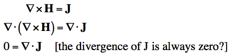 |
[Equation 8] |
|---|
So Equation [8] follows from Equations [6] and [7]. But it says that the divergence of the current density J is always zero. Is this true?
If the divergence of J is always zero, this means that the electric current flowing into any region is always equal to the electric current flowing out of the region (no divergence). This seems somewhat reasonable, as electric current in circuits flows in a loop. But let’s look what happens if we put a capacitor in the circuit:
 Figure 3. A Voltage Applied to A Capacitor.
Now, we know from electric circuit theory that if the voltage is not constant (for example, any periodic wave, such as the 60 Hz voltage that comes out of your power outlets) then current will flow through the capacitor. That is, we have I not equal to zero in Figure 3.
However, a capacitor is basically two parallel conductive plates separated by air. Hence, there is no conductive path for the current to flow through. This means that no electric current can flow through the air of the capacitor. This is a problem if we think about Equation [8]. To show it more clearly, let’s take a volume that goes through the capacitor, and see if the divergence of J is zero:
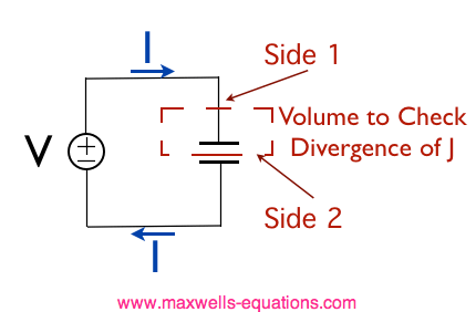 Figure 4. The Divergence of J is not Zero.
In Figure 4, we have drawn an imaginary volume in red, and we want to check if the divergence of the current density is zero. The volume we’ve chosen, has one end (labeled side 1) where the current enters the volume via the black wire. The other end of our volume (labeled side 2) splits the capacitor in half.
We know that the current flows in the loop. So current enters through Side 1 of our red volume. However, there is no electric current that exits side 2. No current flows within the air of the capacitor. This means that current enters the volume, but nothing leaves it – so the divergence of J is not zero. We have just violated our Equation [8], which means the theory does not hold. And this was the state of things, until our friend Maxwell came along.
Maxwell knew that the Electric Field (and Electric Flux Density (D) was changing within the capacitor. And he knew that a time-varying magnetic field gave rise to a solenoidal Electric Field (i.e. this is Farday’s Law – the curl of E equals the time derivative of B). So, why is not that a time varying D field would give rise to a solenoidal H field (i.e. gives rise to the curl of H). The universe loves symmetry, so why not introduce this term? And so Maxwell did, and he called this term the displacement current density:
 |
[Equation 9] |
|---|
This term would “fix” the circuit problem we have in Figure 4, and would make Farday’s Law and Ampere’s Law more symmetric. This was Maxwell’s great contribution. And you might think it is a weak contribution. But the existance of this term unified the equations and led to understanding the propagation of electromagnetic waves, and the proof that all waves travel at the same speed (the speed of light)! And it was this unification of the equations that Maxwell presented, that led the collective set to be known as Maxwell’s Equations. So, if we add the displacement current to Ampere’s Law as written in Equation [6], then we have the final form of Ampere’s Law:
 |
[Equation 10] |
|---|
And that is how Ampere’s Law came into existance!
Intrepretation of Ampere’s Law
So what does Equation [10] mean? The following are consequences of this law:
- A flowing electric current (J) gives rise to a Magnetic Field that circles the current
- A time-changing Electric Flux Density (D) gives rise to a Magnetic Field that circles the D field
Ampere’s Law with the contribution of Maxwell nailed down the basis for Electromagnetics as we currently understand it. And so we know that a time varying D gives rise to an H field, but from Farday’s Law we know that a varying H field gives rise to an E field…. and so on and so forth and the electromagnetic waves propagate – and that’s cool.
This website is educational. Materials within it are being used in accord with the Fair Use doctrine, as defined by United States law.
§107. Limitations on Exclusive Rights: Fair Use
Notwithstanding the provisions of section 106, the fair use of a copyrighted work, including such use by reproduction in copies or phone records or by any other means specified by that section, for purposes such as criticism, comment, news reporting, teaching (including multiple copies for classroom use), scholarship, or research, is not an infringement of copyright. In determining whether the use made of a work in any particular case is a fair use, the factors to be considered shall include:
the purpose and character of the use, including whether such use is of a commercial nature or is for nonprofit educational purposes;
the nature of the copyrighted work;
the amount and substantiality of the portion used in relation to the copyrighted work as a whole; and
the effect of the use upon the potential market for or value of the copyrighted work. (added pub. l 94-553, Title I, 101, Oct 19, 1976, 90 Stat 2546)
Carbon dating
Introduction
“At an archaeological dig, a piece of wooden tool is unearthed – and the archaeologist finds it to be 5,000 years old. A child mummy is found high in the Andes – and the archaeologist says the child lived more than 2,000 years ago. How do scientists know how old an object or human remains are? What methods do they use and how do these methods work?
Carbon-14 dating is a way of determining the age of archaeological artifacts of a biological origin up to about 50,000 years old. It is used in dating things such as bone, cloth, wood and plant fibers that were created in the relatively recent past by human activities.”
- How Stuff Works, How Carbon-14 Dating Works, Marshall Brain
“The method was developed by Willard Libby in the late 1940s and soon became a standard tool for archaeologists. Libby received the Nobel Prize in Chemistry for his work in 1960. ” – Wikipedia
How does it work?
Radiocarbon is constantly being created in the atmosphere by the interaction of cosmic rays with atmospheric nitrogen.

From the matthew2262 wordpress blog.
The resulting radiocarbon combines with atmospheric oxygen to form radioactive carbon dioxide.
That is incorporated into plants by photosynthesis.
Animals then acquire 14 C by eating the plants.
When the animal or plant dies, it stops exchanging carbon with its environment, and from that point onwards the amount of 14 C it contains begins to decrease, as the 14
C undergoes radioactive decay.
Measuring the amount of 14 C in a sample from a dead plant or animal such as a piece of wood or a fragment of bone provides information that can be used to calculate when the animal or plant died.
The older a sample is, the less 14 C there is to be detected, and because the half-life of 14 C (the period of time after which half of a given sample will have decayed) is about 5,730 years.
The oldest dates that can be reliably measured by this process date to around 50,000 years ago, although special preparation methods occasionally permit accurate analysis of older samples.
– Carbon Dating, Wikipedia
****************
As years go by, how much C14 is left?


C12 does not decay and remains constant in a sample, whereas C14 decays at an even, constant rate.
By measuring the ratio of C12 to C14, we can understand how long a sample has been around for.
The half life of C 14 is around 5,730 years. As seen by the second graph, this means that if a sample has half of the C14 it should usually have, it has been around for 5,730 years. A quarter of the amount, double that time, one eight of the original amount, more still.
Carbon dating is only as accurate as the consistency of it’s decay rate, which is unchanging and extremely uniform.
It is almost exclusively used for organic material as all life on earth is carbon based.
There is a misconception that carbon dating is used to date the age of the earth. For longer time scales, other elements are used, based on the same principles.
Graphs from a video by Scientific American that explains carbon dating. Watch the full video here How Does Radiocarbon Dating Work? – Instant Egghead #28: Scientific American
- text from http://blunt-science.tumblr.com/post/109954909373/a-representation-of-the-age-span-carbon-dating-is
_______________________________________________________________________________
Is radiocarbon dating reliable?
Excerpted from National Center for Science Education, by Christopher Gregory Weber:
http://ncse.com/cej/3/2/answers-to-creationist-attacks-carbon-14-dating
Radiocarbon dating can easily establish that humans have been on the earth for over twenty thousand years …. it is one of the most reliable of all the radiometric dating methods.
Question: How does carbon-14 dating work?
Answer:
Cosmic rays in the upper atmosphere are constantly converting the isotope nitrogen-14 (N-14) into carbon-14 (C-14 or radiocarbon).
Living organisms are constantly incorporating this C-14 into their bodies along with other carbon isotopes.
When the organisms die, they stop incorporating new C-14
The old C-14 starts to decay back into N-14 by emitting beta particles.
The older an organism’s remains are, the less beta radiation it emits because its C-14 is steadily dwindling at a predictable rate.
So, if we measure the rate of beta decay in an organic sample, we can calculate how old the sample is. C-14 decays with a half-life of 5,730 years.
______________________________________________________________
Question: Kieth and Anderson radiocarbon-dated the shell of a living freshwater mussel and obtained an age of over two thousand years. ICR creationists claim that this discredits C-14 dating. How do you reply?
Answer: It does discredit the C-14 dating of freshwater mussels, but that’s about all. Kieth and Anderson show considerable evidence that the mussels acquired much of their carbon from the limestone of the waters they lived in and from some very old humus as well.
Carbon from these sources is very low in C-14 because these sources are so old and have not been mixed with fresh carbon from the air. Thus, a freshly killed mussel has far less C-14 than a freshly killed something else, which is why the C-14 dating method makes freshwater mussels seem older than they really are.
When dating wood there is no such problem because wood gets its carbon straight from the air, complete with a full dose of C-14.
____________________________________________________________________
Question: A sample that is more than fifty thousand years old shouldn’t have any measurable C-14. Coal, oil, and natural gas are supposed to be millions of years old; yet creationists say that some of them contain measurable amounts of C-14, enough to give them C-14 ages in the tens of thousands of years. How do you explain this?
Answer: Very simply. Radiocarbon dating doesn’t work well on objects much older than twenty thousand years, because such objects have so little C-14 left that their beta radiation is swamped out by the background radiation of cosmic rays and potassium-40 (K-40) decay.

Younger objects can easily be dated, because they still emit plenty of beta radiation, enough to be measured after the background radiation has been subtracted out of the total beta radiation. However, in either case, the background beta radiation has to be compensated for, and, in the older objects, the amount of C-14 they have left is less than the margin of error in measuring background radiation. As Hurley points out:
Without rather special developmental work, it is not generally practicable to measure ages in excess of about twenty thousand years, because the radioactivity of the carbon becomes so slight that it is difficult to get an accurate measurement above background radiation. (p. 108)
Cosmic rays form beta radiation all the time; this is the radiation that turns N-14 to C-14 in the first place. K-40 decay also forms plenty of beta radiation. Stearns, Carroll, and Clark point out that “. . . this isotope [K-40] accounts for a large part of the normal background radiation that can be detected on the earth’s surface” (p. 84).
This radiation cannot be totally eliminated from the laboratory, so one could probably get a “radiocarbon” date of fifty thousand years from a pure carbon-free piece of tin. However, you now know why this fact doesn’t at all invalidate radiocarbon dates of objects younger than twenty thousand years and is certainly no evidence for the notion that coals and oils might be no older than fifty thousand years.
____________________________________________________________________________________________
Question: Creationists such as Cook (1966) claim that cosmic radiation is now forming C-14 in the atmosphere about one and one-third times faster than it is decaying. If we extrapolate backwards in time with the proper equations, we find that the earlier the historical period, the less C-14 the atmosphere had.
If we extrapolate as far back as ten thousand years ago, we find the atmosphere would not have had any C-14 in it at all. If they are right, this means all C-14 ages greater than two or three thousand years need to be lowered drastically and that the earth can be no older than ten thousand years. How do you reply?
Answer: Yes, Cook is right that C-14 is forming today faster than it’s decaying. However, the amount of C-14 has not been rising steadily as Cook maintains; instead, it has fluctuated up and down over the past ten thousand years. How do we know this? From radiocarbon dates taken from bristlecone pines. There are two ways of dating wood from bristlecone pines: one can count rings or one can radiocarbon-date the wood.
Since the tree ring counts have reliably dated some specimens of wood all the way back to 6200 BC, one can check out the C-14 dates against the tree-ring-count dates. Admittedly, this old wood comes from trees that have been dead for hundreds of years, but you don’t have to have an 8,200-year-old bristlecone pine tree alive today to validly determine that sort of date. It is easy to correlate the inner rings of a younger living tree with the outer rings of an older dead tree. The correlation is possible because, in the Southwest region of the United States, the widths of tree rings vary from year to year with the rainfall, and trees all over the Southwest have the same pattern of variations.
When experts compare the tree-ring dates with the C-14 dates, they find that radiocarbon ages before 1000 BC are really too young—not too old as Cook maintains. For example, pieces of wood that date at about 6200 BC by tree-ring counts date at only 5400 BC by regular C-14 dating and 3900 BC by Cook’s creationist revision of C-14 dating (as we see in the article, “Dating, Relative and Absolute,” in the Encyclopaedia Britannica). So, despite claims, C-14 before three thousand years ago was decaying faster than it was being formed and C-14 dating errs on the side of making objects from before 1000 BC look too young, not too old.
_______________________________________________________________
Question: But don’t trees sometimes produce more than one growth ring per year? Wouldn’t that spoil the tree-ring count?
Answer: If anything, the tree-ring sequence suffers far more from missing rings than from double rings. This means that the tree-ring dates would be slightly too young, not too old.

Of course, some species of tree tend to produce two or more growth rings per year. But other species produce scarcely any extra rings. Most of the tree-ring sequence is based on the bristlecone pine. This tree rarely produces even a trace of an extra ring; on the contrary, a typical bristlecone pine has up to 5 percent of its rings missing. Concerning the sequence of rings derived from the bristlecone pine, Ferguson says:
In certain species of conifers, especially those at lower elevations or in southern latitudes, one season’s growth increment may be composed of two or more flushes of growth, each of which may strongly resemble an annual ring.
Such multiple growth rings are extremely rare in bristlecone pines, however, and they are especially infrequent at the elevation and latitude (37� 20′ N) of the sites being studied. In the growth-ring analyses of approximately one thousand trees in the White Mountains, we have, in fact, found no more than three or four occurrences of even incipient multiple growth layers. (p. 840)
In years of severe drought, a bristlecone pine may fail to grow a complete ring all the way around its perimeter; we may find the ring if we bore into the tree from one angle, but not from another. Hence at least some of the missing rings can be found. Even so, the missing rings are a far more serious problem than any double rings.
Other species of trees corroborate the work that Ferguson did with bristlecone pines. Before his work, the tree-ring sequence of the sequoias had been worked out back to 1250 BC. The archaeological ring sequence had been worked out back to 59 BC. The limber pine sequence had been worked out back to 25 BC.
The radiocarbon dates and tree-ring dates of these other trees agree with those Ferguson got from the bristlecone pine. But even if he had had no other trees with which to work except the bristlecone pines, that evidence alone would have allowed him to determine the tree-ring chronology back to 6200 BC. …
______________________________________________________________________
Question: Does outside archaeological evidence confirm the C-14 dating method?
Answer: Yes. When we know the age of a sample through archaeology or historical sources, the C-14 method (as corrected by bristlecone pines) agrees with the age within the known margin of error.
For instance, Egyptian artifacts can be dated both historically and by radiocarbon, and the results agree. At first, archaeologists used to complain that the C-14 method must be wrong, because it conflicted with well-established archaeological dates; but, as Renfrew has detailed, the archaeological dates were often based on false assumptions.
One such assumption was that the megalith builders of western Europe learned the idea of megaliths from the Near-Eastern civilizations. As a result, archaeologists believed that the Western megalith-building cultures had to be younger than the Near Eastern civilizations.
Many archaeologists were skeptical when Ferguson’s calibration with bristlecone pines was first published, because, according to his method, radiocarbon dates of the Western megaliths showed them to be much older than their Near-Eastern counterparts.
However, as Renfrew demonstrated, the similarities between these Eastern and Western cultures are so superficial that the megalith builders of western Europe invented the idea of megaliths independently of the Near East. So, in the end, external evidence reconciles with and often confirms even controversial C-14 dates.

One of the most striking examples of different dating methods confirming each other is Stonehenge. C-14 dates show that Stonehenge was gradually built over the period from 1900 BC to 1500 BC, long before the Druids, who claimed Stonehenge as their creation, came to England.
Astronomer Gerald S. Hawkins calculated with a computer what the heavens were like back in the second millennium BC, accounting for the precession of the equinoxes, and found that Stonehenge had many significant alignments with various extreme positions of the sun and moon (for example, the hellstone marked the point where the sun rose on the first day of summer). Stonehenge fits the heavens as they were almost four thousand years ago, not as they are today, thereby cross-verifying the C-14 dates.
Textbooks
Relative Ages of Rocks: WIkiBooks
(WikiBooks: A project hosted by the Wikimedia Foundation for the creation of free content textbooks)
http://en.wikibooks.org/wiki/High_School_Earth_Science/Relative_Ages_of_Rocks
http://en.wikibooks.org/wiki/High_School_Earth_Science/Absolute_Ages_of_Rocks
External links
Willard Libby and Radiocarbon Dating. American Chemical Society
Learning Standards
A Framework for K-12 Science Education: Practices, Crosscutting Concepts, and Core Ideas (2012), from the National Research Council of the National Academies.
By the end of grade 12. Radioactive decay lifetimes and isotopic content in rocks provide a way of dating rock formations and thereby fixing the scale of geological time.
College Board Standards for College Success: Science
ES.3 Earth’s History: Relative and Absolute dating. Students understand that various dating methods — relative and absolute — have been used to determine the age of Earth.
Suggested Connections. Between Earth Science and Other Disciplines: Evidence of Common Ancestry and Divergence (LS.1.1); Living Systems and the Physical Environment (LS.3.1); Nuclear Chemistry (C.1.6); Nuclear Interactions and the Conservation of Mass–Energy (P.2.3)
Benchmarks: American Association for the Advancement of Science.
Knowledge of radioactivity helps them understand how rocks can be dated, which helps them appreciate the scale of geologic time… Scientific evidence indicates that some rock layers are several billion years old. 4C/H6** (BSL)
Peptide bonds – How we make proteins
2 amino acids can join to form a peptide.
A very long peptide is known as a protein.
When they join one of the amino acid’s loses an H atom, while the other loses an OH moiety (part of a molecule) They join together to form H2O (water.) This is a condensation reaction.

Doc Kaiser’s Microbiology Home Page (Gary E. Kaiser)
Here is another animation of the same process
The CONH link created is called a peptide bond (red)
Water (blue) is removed.
This process can be continued repeatedly to form longer peptides (eventually, when they are over 50 amino acids long, we call them proteins.)

BioTopics.co.uk by Richard Steane
The monomer here is an amino acid.
The polymer here is a peptide or protein.
These are 20 different types of common amino acids.
Amino acids are bonded together to make peptides, or proteins.
A peptide is just a small protein, less than 50 amino acids (aa) long.
Proteins are much larger, 100 aa, 500 aa, even 1,000 aa.
A chain of amino acids folds up into a shape.
Every protein has its own shape.

If all land ice melted how would coastlines change
Sea level rise in the last century
This image from High-tide flood risk is accelerating, putting coastal economies at risk, Renee Collini, The Conversation, 6/14/2021, Coastal Climate Resilience Specialist, NOAA Sea Grant, Mississippi State University.
She writes
As sea level rises, it can be easy to miss the subtlety of higher water. It’s much harder to overlook saltwater more frequently flooding streets, impeding daily life and making existing problems worse.
The frequency of high-tide flooding along the U.S. coasts has doubled since 2000, and it’s expected to increase five to 15 times more in the next 30 years, the National Oceanic and Atmospheric Administration warns in a new report released July 14, 2021.
I work with coastal communities in the northern Gulf of Mexico that are facing the risks of rising seas as they try to avoid preventable damages and costs, such as infrastructure failures and falling property values. Information like the NOAA report is critical to helping these communities succeed.
Last year, the U.S. averaged four days of high-tide flooding, but that number doesn’t tell the whole story – regionally, several areas saw far more. There were record-breaking numbers of high-tide flooding days in 2020 along the Gulf of Mexico and southeast Atlantic coasts. The city of Bay St. Louis, Mississippi, jumped from three days of high-tide flooding in 2000 to 22 days in 2020.

Sea level changes over last 10,000 years
Scientists have used evidence to reconstruct sea-level rise around America’s northeast coast over the last 10,000 years.
New Jersey going back 10,000 years in research newly published in the Journal of Quaternary Science. To do this, they collected sediment cores drilled tens of meters below ground from coastal marshes, then examined the sediment back in a lab for microscopic organisms that only exist at specific depths below sea level. Salt marsh grasses also fossilized within the sediment were used to radiocarbon-date the samples.
The 10 maps contained in the GIF below show the movement of sea level at 1,000-year intervals leading up today:
https://www.citylab.com/environment/2013/05/if-gif-10000-years-sea-level-rise-doesnt-freak-you-out-nothing-will/5751/

HORTON, B. P., ENGELHART, S. E., HILL, D. F., KEMP, A. C., NIKITINA, D., MILLER, K. G. and PELTIER, W. R. (2013), Influence of tidal-range change and sediment compaction on Holocene relative sea-level change in New Jersey, USA. J. Quaternary Sci., 28: 403–411
If This GIF of 10,000 Years of Sea Level Rise Doesn’t Freak You Out, Nothing Wil
Boston
Boston underwater: How the rising sea levels will affect the city
Also
What Could Disappear. New York Times Sunday Review.
Quote
“If we keep burning fossil fuels indefinitely, global warming will eventually melt all the ice at the poles and on mountaintops, raising sea level by 216 feet. Explore what the world’s new coastlines would look like.
“The maps here show the world as it is now, with only one difference: All the ice on land has melted and drained into the sea, raising it 216 feet and creating new shorelines for our continents and inland seas.
There are more than five million cubic miles of ice on Earth, and some scientists say it would take more than 5,000 years to melt it all. If we continue adding carbon to the atmosphere, we’ll very likely create an ice-free planet, with an average temperature of perhaps 80 degrees Fahrenheit instead of the current 58.”
from National Geographic Magazine, What the World Would Look Like if All the Ice Melted
Map 1
The entire Atlantic seaboard would vanish, along with Florida and the Gulf Coast. In California, San Francisco’s hills would become a cluster of islands and the Central Valley a giant bay. The Gulf of California would stretch north past the latitude of San Diego—not that there’d be a San Diego.

Map 2
The Amazon Basin in the north and the Paraguay River Basin in the south would become Atlantic inlets, wiping out Buenos Aires, coastal Uruguay, and most of Paraguay. Mountainous stretches would survive along the Caribbean coast and in Central America.

Map 3
London? A memory. Venice? Reclaimed by the Adriatic Sea. Thousands of years from now, in this catastrophic scenario, the Netherlands will have long since surrendered to the sea, and most of Denmark will be gone too. Meanwhile, the Mediterranean’s expanding waters will also have swelled the Black and Caspian Seas.

Map 3
Land now inhabited by 600 million Chinese would flood, as would all of Bangladesh, population 160 million, and much of coastal India. The inundation of the Mekong Delta would leave Cambodia’s Cardamom Mountains stranded as an island.

Map
East Antarctica: The East Antarctica ice sheet is so large—it contains four-fifths of all the ice on Earth—that it might seem unmeltable. It survived earlier warm periods intact. Lately it seems to be thickening slightly—because of global warming.
The warmer atmosphere holds more water vapor, which falls as snow on East Antarctica. But even this behemoth is unlikely to survive a return to an Eocene Climate.
West Antarctica: Like the Greenland ice sheet, the West Antarctic one was apparently much smaller during earlier warm periods. It’s vulnerable because most of it sits on bedrock that’s below sea level.The warming ocean is melting the floating ice sheet itself from below, causing it to collapse. Since 1992 it has averaged a net loss of 65 million metric tons of ice a year.

All maps here by: Jason Treat, Matthew Twombly, Web Barr, Maggie Smith, NGM Staff. Art Kees Veenebos. From Sept. 2013 National Geographic Society
What the World Would Look Like if All the Ice Melted (National Geographic)
.
Latest Posts
-

Importance of art education
Why is teaching art intrinsically important to being human? Some would have us believe that we should have art education in our schools because it…
-

What are broken symmetries?
Symmetry is an important concept for understanding how our universe works. Symmetry lets us see what stays the same when certain conditions change. Symmetries are…
-

Native Americans in New England
When did the ancestors of native Americans arrive in what we now call New England? Their earliest confirmed presence in New England is about 12,000–13,000…
-
Why is music education important
Why is music intrinsically important to being human? Every year I read yet another article trying to persuade us that we should have music education…
